
RMS Amplitude Attributes
The figure above let us see the difference of the cross seismic section after the RMS attribute is applied. At inline 732, the upper part shows higher amplitude in the RMS amplitude in 3D volume attribute especially at the area of the bright spot. High amplitude in RMS attribute represents either the spot has potential in hydrocarbon or it could also indicate lithological boundary with high acoustic impedance. From our seismic section, we can assume that the high amplitude indicates that the lithology might change from low acoustic impedance to high acoustic impedance. The high acoustic impedance is most probably the reservoir rock that has hydrocarbon. The high amplitude in this seismic section can be seen in one curvy horizon and also at the almost top horizon. The high amplitude present at the almost top horizon might be due to the hydrocarbon that escape through the faulted curvy horizon.
RMS stands for “Root Mean Square”. It is a post-stack attribute that evaluate the square root of the sum of squared amplitudes divided by the number of samples within the specified window used. The energy content of the given seismic section can be observed by applying this RMS attribute on the original seismic section. It helps to locate the Direct Hydrocarbon Indicator (DHI). This is because the RMS amplitude is closely related to the porosity of the region. It means that region with high RMS amplitude is most probably a high porosity lithology. As reservoir rock is known as a rock that is high in porosity, DHI always give high amplitude RMS.
Figure 2: show the comparison of seismic cross section at inline 732 between the original seismic data and the RMS amplitude in 3D volume attribute.
In our seismic section, we can see a region that shows a pull up effect within the crossline range of 2406 to 2526 . It is initiated by faults as seen in the image (A). The left side of the faulted high RMS amplitude horizon is then showing a pull down effect. It can be seen in image (B). However, during the pull time effect, the high RMS amplitude is slowly reducing before it disappears.
Figure 3: shows seismic cross section of RMS amplitude in volume attribute at crossline 1658. In this figure, the high amplitude that is located at the top of the cross seismic section can be clearly seen. The high RMS amplitude that is located at the top of the cross seismic section can be seen within the crossline range from 1748 to 1608.
Figure 4: shows seismic cross section of RMS amplitude in volume attribute at crossline 2188. In this figure, we can see the high RMS amplitude horizon is faulted.
Figure 10: shows the surface RMS amplitude of Horizon 4. At this horizon, there are lesser areas showing high RMS amplitude. The top of this horizon is taken from time slice of -2270 and the bottom part of this horizon time slice of -2970.
Figure 5: shows the cross seismic section of RMS amplitude in 3D volume attribute. The image labelled as (A) is the seismic section at crossline 2296, (B) is the seismic section at crossline 2386 and ( C ) is the seismic section at crossline 2446.
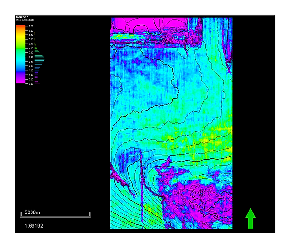
Figure 7: shows the surface RMS amplitude of Horizon 1. The high RMS amplitude can hardly be seen at this horizon. The top of this horizon is taken from time slice of -370 and the bottom part of this horizon is at time slice of -510.
Figure 6: shows the cross seismic section of RMS amplitude in timeslice attribute. From the image labelled as A, B and C, the high RMS amplitude can be seen propagating from North West direction to the South East direction. ( A : Z = -1206, B : Z = -1186, C : Z = -1076).
Figure 11: shows the surface RMS amplitude of Horizon 5.This horizon has the least areas showing high RMS amplitude. The top of this horizon is taken from time slice of -2630 and the bottom part of this horizon is at time slice of -3530.
Figure 8: shows the surface RMS amplitude of Horizon 2. At this horizon, the high RMS amplitude can be seen at the upper part of the image. It is showing high RMS amplitude at the low elevation area. This horizon is showing the high RMS amplitude coefficients. The top of this horizon is taken from time slice of -870 and the bottom part of this horizon is at time slice of -1230.
Figure 9: shows the surface RMS amplitude of Horizon 3. At this horizon, the high RMS amplitude can be seen at the right side of the image. The area it shows high RMS amplitude is scattered within high elevation area to low elevation area. The RMS amplitude is reduced compared to RMS amplitude shown at horizon 2. The top of this horizon is taken from time slice of -1390 and the bottom part of this horizon is at time slice of -1860.